Computing Logic Funcitons using Perceptrons
Emulated Neurons
Neural networks are built on units called neurons, and for this exercise a special neuron called a perceptron is used. Perceptrons are special in that they can represent fundamental logic functions: AND, OR, NAND, NOR. Though a perceptron can’t represent XAND or XOR, layered perceptrons can, thus all logic functions can potentially be built using a layered network structure.
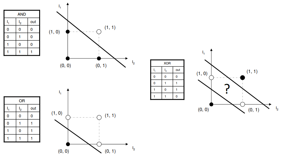
images showing perceptrons' logic structure
Perceptrons work by multiplying a vector of inputs by a weight vector and passing the sum of that input-weight vectors through an activation function. For this exercise I used the sigmoid function, but there are many others. Weights are [nxm] matrices, where n is the dimension of the input and m is the dimension of the output.
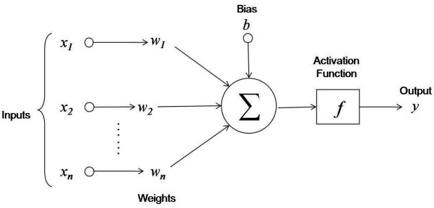
image showing perceptron model
Here is a sketch algorithm to implement a perceptron node:
\(\Sigma (x_iw_i ) = x_1w_1 + x_2 w_2 + ... + x_nw_n\)
\(\sigma = \frac{1}{1+e^{\Sigma (x_iw_i )}}\)
- x is the sample input
- w is the the associated weight for the input sample
For the perceptron to work properly, the weights need to be adjusted according to the desired output. To calculate and adjust the error we first subtract the predicted output from the actual output.
\(\epsilon=y-\sigma\)
- ϵ is the error
- y is the acutal output
- σ is defined above
Using gradient descent, we find the adjustment needed for the weights by computing the derivative of the sigmoid function and multiplying that by the error to give us the final adjustment for the weights:
\(\sigma' = \sigma (1- \sigma)\)
- σ’ is the sigmoid derivative when given σ as above
\(adjustment = \epsilon*\sigma'\)
Networked together, perceptrons can be immensely powerful and are the foundations by which many neural nets are built. These new weights wouldn’t have changed much, but over many iterations they converge to their proper values of minimizing error. This method of adjusting the weights is called backpropagation.
To test the algorithm a small, simple sample set was used to provide easy-to-interpret results. The table below shows the following dataset such that the output is 1 if first or second columns contained a 1, disregrading the third column:
| Variable 1 | Variable 2 | Variable 3 | Output | |
|---|---|---|---|---|
| Input 1 | 0 | 0 | 1 | 0 |
| Input 2 | 1 | 1 | 1 | 1 |
| Input 3 | 1 | 0 | 1 | 1 |
| Input 4 | 0 | 1 | 1 | 1 |
perceptron.py demonstrates the algorithm and predicted output. Given the input array and initial weights adjusted 200 times, the predicted results are as follows:
| Variable 1 | Variable 2 | Variable 3 | Output | |
|---|---|---|---|---|
| Input 1 | 0 | 0 | 1 | 0.135 |
| Input 2 | 1 | 1 | 1 | 0.999 |
| Input 3 | 1 | 0 | 1 | 0.917 |
| Input 4 | 0 | 1 | 1 | 0.917 |
Given an infinite number of iterations the algorithm would converge to either 0 or 1, but in 200 iterations our results are close enough to see a clear distinction.
Applied to a larger dataset, classifier.py, we can create a linear classifier.
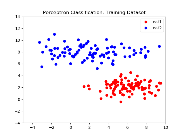
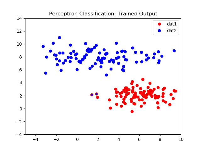
Left: Initial 2D dataset, Right: Perceptron classifier results

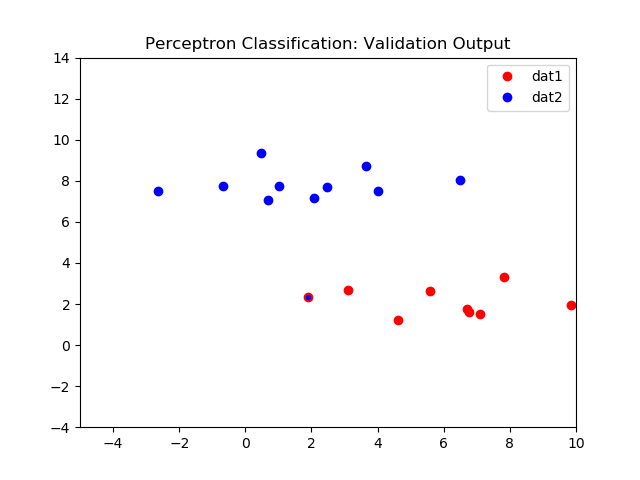
Left: Initial validation dataset, Right: Perceptron validation classifier results
The graph below shows the network error over 500 iterations. As expected the initial error is very high due to the weights being initially random. The error quicky drops after ~30 iterations, but never quite reaches zero. In this case error is ~4%, reflected in the misclassifed samples in both images on the right.
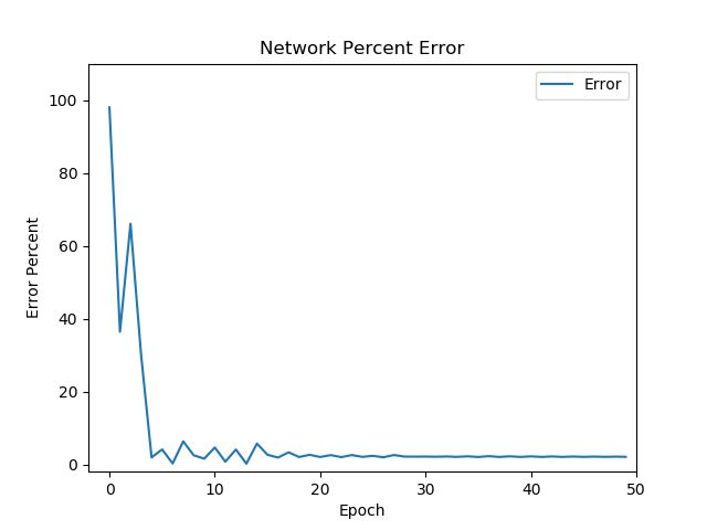
Network error percentage drops after each epoch, indicating a model is being learned