Microscopy and Image Analysis
FIJI
FIJI is an open source image analysis tool for the scientific community. This post demos how to use some of the tools FIJI has, including data collection techniques.
Initial Data
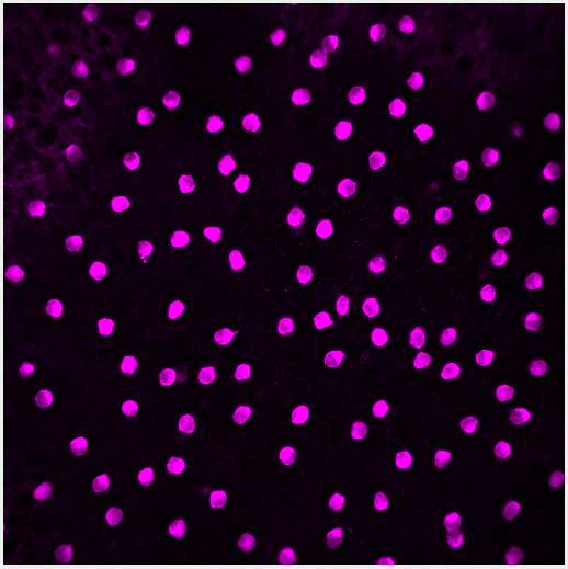
The image for this demo is of starburst amacrine cells (SACs), interneurons in the retina. The image is a single channel .tif, 512x512 pixels, with each pixel representing 0.62 microns. With this information we definitively measure how big each cell is.
Brightness & Contrast
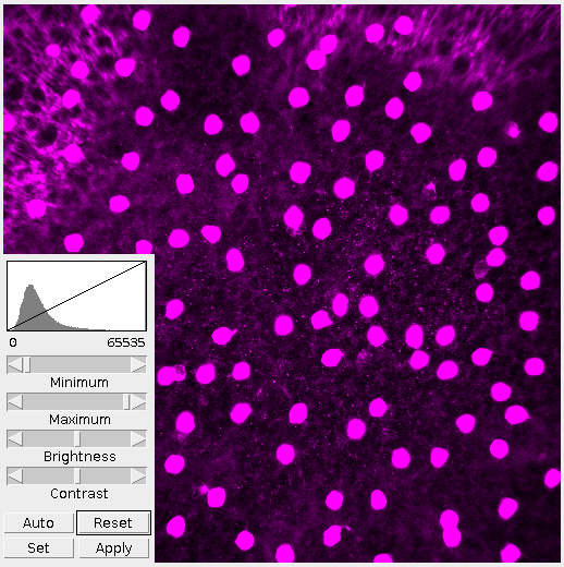
The first thing I do is adjust the brightness and contrast. By looking at the histogram we can see that the image is very dark, more dark than it needs to be. Lowering the maximum value fills out the range of present colors. The difference is clear in Figure 2.
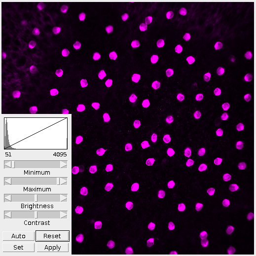
It’s important in this step to not over-saturate the image by raising or lowering the minimum/maximum values. This step is to present the information within the image as a whole. Tweaking and refining will come later.
For this demo I want to look at the cells, not the nebulous background or nodelets. Given that, the image doesn’t need to be as bright. However, it’s important to note that brightening the image revealed more cells and provided better definition. Where this middle ground is depends on the observer and whatever their interests are.
Threshold
Thresholding is an important first step in many image analysis techniques. It converts the image to a black and white image. Here I adjust the histogram in the same fashion as before and focus it around the peak. That filters out the background while keeping true to the cell size and shape.
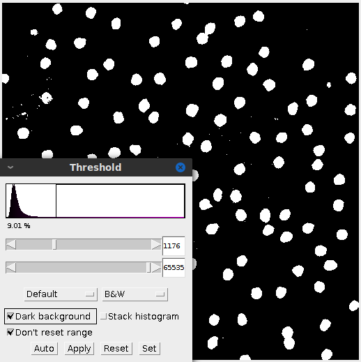
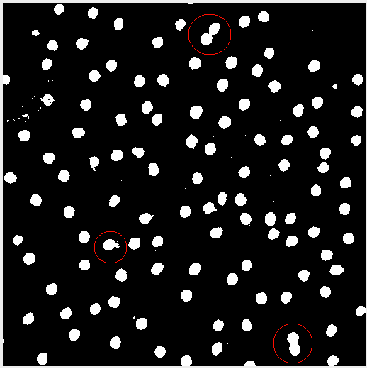
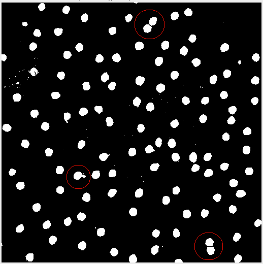
Sometimes after adjusting the image, the subject matter may blend together. In this case applying the threshold created some peanut shaped objects. Watershed segmentation addresses the issue and cuts the “peanut” in half. Figure 4 highlights the effect.
Analyzing the Image
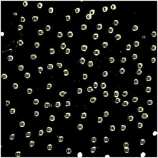
This is where the magic happens. Once the cells are properly individualized we can count and measure each cell. FIJI automatically does this. Since I’m interested in the size and position of the cells I’ve excluded any cells that are cropped by the edge. From here the data is exported to a .csv file.
MATLAB
The exported data contains a cell ID, area, and x/y position. First, I want to determine if the size of the cells fits any distribution. The Jarque-Bera Test tests the normality of a dataset and MATLAB has a built in function for this. Applying the JB test to the data gives a result of 1, meaning that the test rejects the hypothesis that the data (cell size) is normally distributed.
We can also look at the nearest neighbor of each cell (see Figure 6).
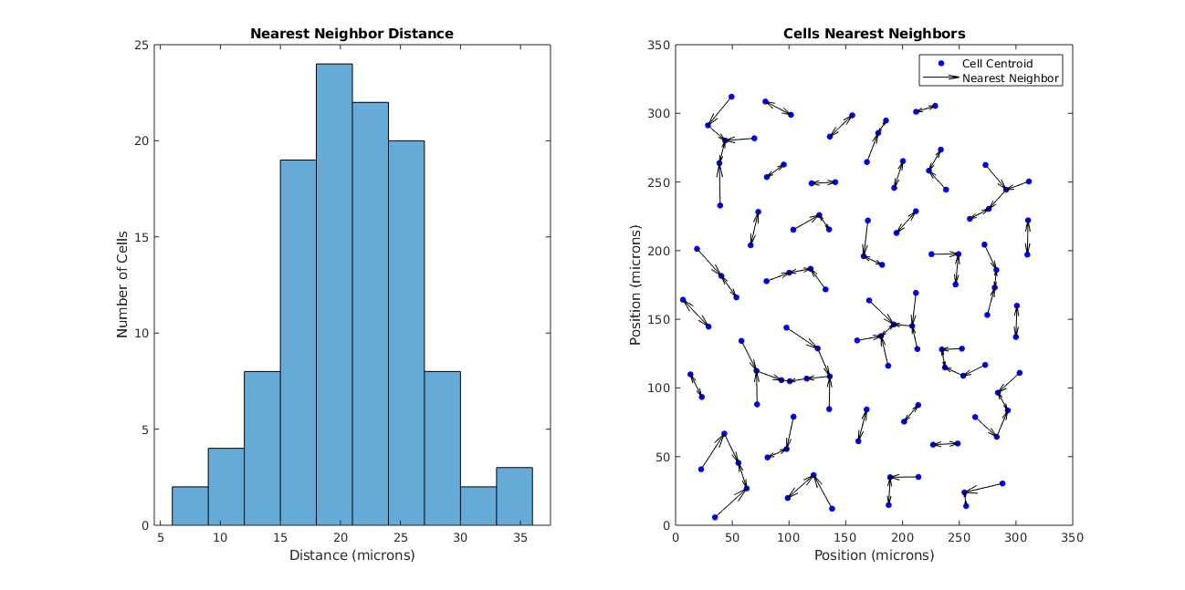
So the size of the cells aren’t interesting, but what about the spatial distribution of the cells? Using the data provided by the image, we can calculate the coefficient of variation:
μ = 21.0440
σ = 5.3968
CoV = σ/μ = 0.26
(units are in microns)
Defining λ as the average distance of the nearest neighbor (21.0440), the Poisson coefficient of variation is:
CoV = λ^(-1/2) = 0.22
A Poisson distribution assumes that cells are “blind” to each other’s positions as they develop and can’t occupy the same space. The fact that these coefficients are close infers that these SACs are also blind as they develop.